Algorithmic self-assembly

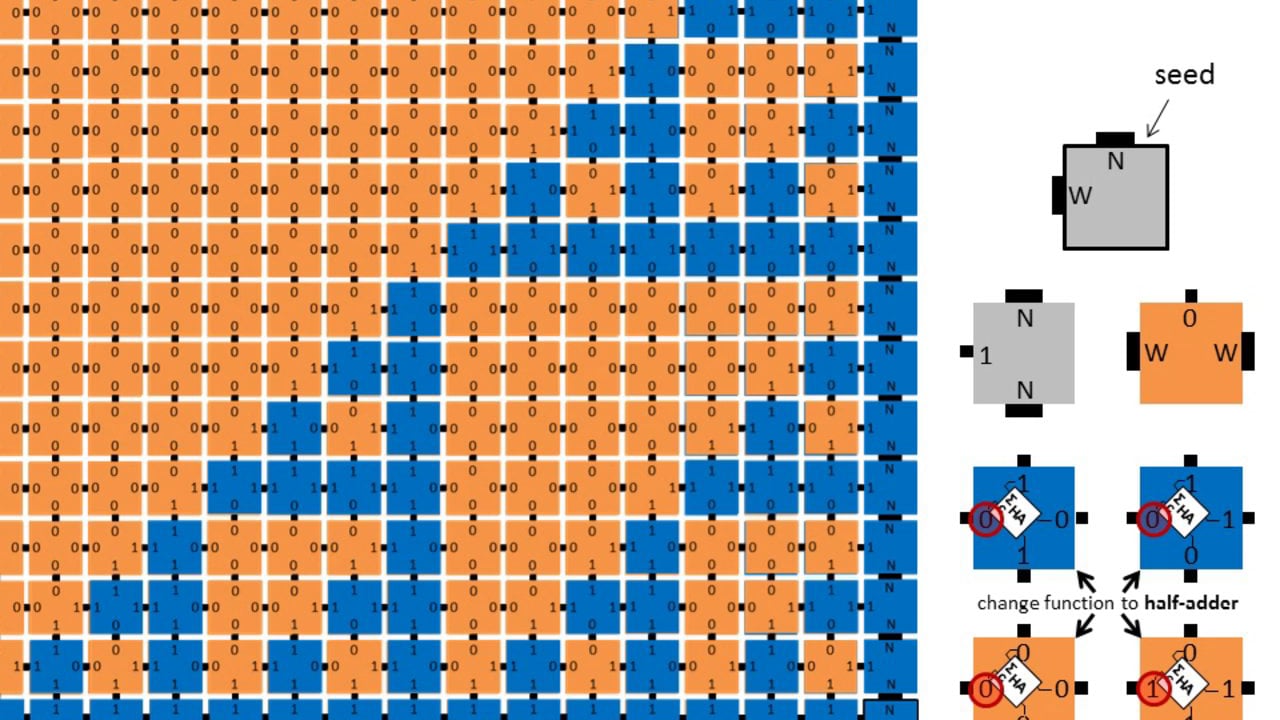
Self-assembly is a process in which smaller components (primitives) self-assemble into more complex shapes. Every component in the system is completely independent of others. Components obey very simple rules with which we can guide the self-assembly process to obtain desired shapes.

The process of self-assembly can be observed in nature i.e Chemistry (links between molecules), biology (lipids self-assemble into a cell membrane). In nature, these processes happen completely in parallel. The molecules move around the space trying to find a stable link. Consequently, they merge into a more complex shape.

The scientific question is weather we can adjust the laws by which these natural processes happen in-vitro. By doing this, we could basically program the rules and inherently define the problem where the final shape would be the solution. If this was possible, we could potentially find solutions to problems which are so hard, no computer can find a solution. Such a system would reduce the problem size by using nature's \"infinite\" parallelism. Granted, we are far from an actual physical test. There are still a lot of hurdles to overcome such as scaling, defining problems, reading results, etc.. However, we can simulate the process and define problems in the simulator. If the assumptions the simulator makes are correct, we could have a number of problems already constructed once the experiments with are done on biological and chemical systems.

The answers to the above problems are outside the scope of this course. However, we can learn a lot by simulating the process of self-assembly. Your task is to implement a simulator with a given configuration of components self-assembles into the final shape. The simulator will be capable of real-time rendering to observe the process and the final shape.

This project should be considered by students comfortable with research oriented tasks. More details can be found at http://www.dna.caltech.edu/Papers/algorithmic_tiles2012doty.pdf

Implementation guidelines

1. Implementation of the graphical interface:

   • The drawing of the graphics should be done independently of the computational threads.

   • The default size of the window is 800x600px but can be adjusted manually.

   • The graphical interface must be implemented in JavaFx.

   • The graphical interface can scale, zoom and move. Initially, it scales to fit all points in the view-port.

2. Running the program:

   • The program can be ran in different modes (sequential, parallel, distributed) by specifying a parameter.

   • The program measures run-time needed to complete.

3. Problem specific implementation requirements

   • Rendering should not be considered in measuring runtime.

   • The implementation must adapt automatically to the hardware it is being ran on (Physical CPU's, Cores, Memory, etc..);

Testing

The report must include extensive testing and explanation of results (numeric and graphical). To test the performance of different implementations a tile configuration must be chosen, such that the computation takes a lot of time. An example would be a Sierpinski triangle tile configuration. Increase the size of the formation gradually to show how all three solutions scale relative to the problem size. The report must detail how the tests were performed coupled with the results(numerical and graphical). Explain the results in detail.